Datei:Lastprofil EWE Frühjahr mit Kraftwerkseinsatz schematisch.svg

Originaldatei (SVG-Datei, Basisgröße: 900 × 720 Pixel, Dateigröße: 129 KB)
![]()
Diese Datei und die Informationen unter dem roten Trennstrich werden aus dem zentralen Medienarchiv Wikimedia Commons eingebunden.
![]()
Beschreibung
| Beschreibung |
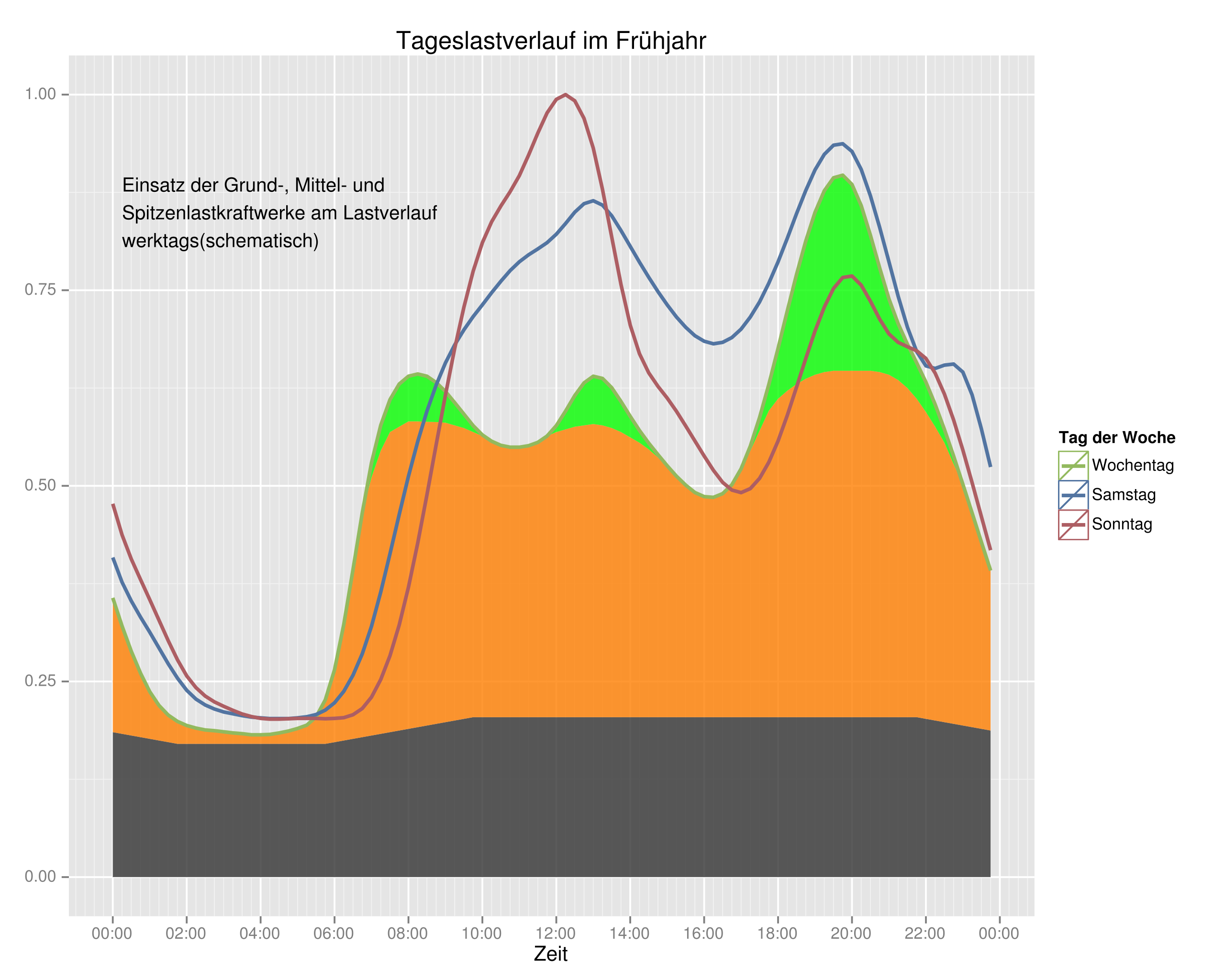
Deutsch: Auf der Basis des Lastprofiles EWE für den Frühlingsanfang wurde schematisch der Einsatz von Grund-, Mittel- und Spitzenlastkraftwerken dargestellt |
| Datum | |
| Quelle | Eigenes Werk |
| Urheber | Karsten Adam |
| Andere Versionen |
 |
Grundlage bildet die Grafik: "Lastprofil VDEW Winter mit Kraftwerkseinsatz schematisch.jpg", eingestellt von "Joes-Wiki"
Data
Download data from EWE AG, unzip, extract worksheet H0 and save file as Lastprofil_H0_2014.csv.
Alternatively use the following data merged into one csv file with two columns.
,H0 Zeitstempel,kWh 19.03.2014 00:00,20.95603 19.03.2014 00:15,18.850222 19.03.2014 00:30,16.954046 19.03.2014 00:45,15.308834 19.03.2014 01:00,13.914587 19.03.2014 01:15,12.882844 19.03.2014 01:30,12.157836 19.03.2014 01:45,11.683792 19.03.2014 02:00,11.377057 19.03.2014 02:15,11.181863 19.03.2014 02:30,11.042438 19.03.2014 02:45,10.986668 19.03.2014 03:00,10.903013 19.03.2014 03:15,10.819358 19.03.2014 03:30,10.763588 19.03.2014 03:45,10.679934 19.03.2014 04:00,10.679934 19.03.2014 04:15,10.707819 19.03.2014 04:30,10.819358 19.03.2014 04:45,10.958783 19.03.2014 05:00,11.153978 19.03.2014 05:15,11.404942 19.03.2014 05:30,12.018411 19.03.2014 05:45,13.301118 19.03.2014 06:00,15.559799 19.03.2014 06:15,18.961762 19.03.2014 06:30,23.088734 19.03.2014 06:45,27.327245 19.03.2014 07:00,31.091713 19.03.2014 07:15,33.908092 19.03.2014 07:30,35.832153 19.03.2014 07:45,37.003321 19.03.2014 08:00,37.588905 19.03.2014 08:15,37.756214 19.03.2014 08:30,37.588905 19.03.2014 08:45,37.114861 19.03.2014 09:00,36.445622 19.03.2014 09:15,35.609074 19.03.2014 09:30,34.74464 19.03.2014 09:45,33.880207 19.03.2014 10:00,33.183084 19.03.2014 10:15,32.70904 19.03.2014 10:30,32.402305 19.03.2014 10:45,32.26288 19.03.2014 11:00,32.26288 19.03.2014 11:15,32.37442 19.03.2014 11:30,32.625385 19.03.2014 11:45,33.099429 19.03.2014 12:00,33.880207 19.03.2014 12:15,34.96772 19.03.2014 12:30,36.138888 19.03.2014 12:45,37.086976 19.03.2014 13:00,37.588905 19.03.2014 13:15,37.421595 19.03.2014 13:30,36.724471 19.03.2014 13:45,35.692729 19.03.2014 14:00,34.577331 19.03.2014 14:15,33.517703 19.03.2014 14:30,32.569615 19.03.2014 14:45,31.705182 19.03.2014 15:00,30.868633 19.03.2014 15:15,30.087855 19.03.2014 15:30,29.418616 19.03.2014 15:45,28.860917 19.03.2014 16:00,28.554183 19.03.2014 16:15,28.498413 19.03.2014 16:30,28.777262 19.03.2014 16:45,29.446501 19.03.2014 17:00,30.645554 19.03.2014 17:15,32.346535 19.03.2014 17:30,34.493676 19.03.2014 17:45,36.975436 19.03.2014 18:00,39.680276 19.03.2014 18:15,42.496655 19.03.2014 18:30,45.229379 19.03.2014 18:45,47.739024 19.03.2014 19:00,49.886165 19.03.2014 19:15,51.503492 19.03.2014 19:30,52.479465 19.03.2014 19:45,52.67466 19.03.2014 20:00,51.977536 19.03.2014 20:15,50.388094 19.03.2014 20:30,48.157299 19.03.2014 20:45,45.703424 19.03.2014 21:00,43.388973 19.03.2014 21:15,41.520682 19.03.2014 21:30,39.98701 19.03.2014 21:45,38.592763 19.03.2014 22:00,37.142746 19.03.2014 22:15,35.469649 19.03.2014 22:30,33.601358 19.03.2014 22:45,31.593642 19.03.2014 23:00,29.474386 19.03.2014 23:15,27.327245 19.03.2014 23:30,25.15222 19.03.2014 23:45,23.005079 |
22.03.2014 00:00,23.984788 22.03.2014 00:15,22.135976 22.03.2014 00:30,20.728327 22.03.2014 00:45,19.513884 22.03.2014 01:00,18.382244 22.03.2014 01:15,17.195403 22.03.2014 01:30,16.008561 22.03.2014 01:45,14.932124 22.03.2014 02:00,14.021292 22.03.2014 02:15,13.358868 22.03.2014 02:30,12.917253 22.03.2014 02:45,12.613642 22.03.2014 03:00,12.392835 22.03.2014 03:15,12.25483 22.03.2014 03:30,12.116825 22.03.2014 03:45,12.006421 22.03.2014 04:00,11.951219 22.03.2014 04:15,11.896017 22.03.2014 04:30,11.896017 22.03.2014 04:45,11.896017 22.03.2014 05:00,11.951219 22.03.2014 05:15,12.034022 22.03.2014 05:30,12.199628 22.03.2014 05:45,12.530839 22.03.2014 06:00,13.082859 22.03.2014 06:15,13.938489 22.03.2014 06:30,15.152931 22.03.2014 06:45,16.753787 22.03.2014 07:00,18.82386 22.03.2014 07:15,21.39075 22.03.2014 07:30,24.261251 22.03.2014 07:45,27.214554 22.03.2014 08:00,30.085055 22.03.2014 08:15,32.679546 22.03.2014 08:30,34.970426 22.03.2014 08:45,36.930095 22.03.2014 09:00,38.586153 22.03.2014 09:15,39.9386 22.03.2014 09:30,41.07024 22.03.2014 09:45,42.063875 22.03.2014 10:00,42.947106 22.03.2014 10:15,43.857938 22.03.2014 10:30,44.713568 22.03.2014 10:45,45.513996 22.03.2014 11:00,46.176419 22.03.2014 11:15,46.700837 22.03.2014 11:30,47.142453 22.03.2014 11:45,47.611669 22.03.2014 12:00,48.246492 22.03.2014 12:15,49.04692 22.03.2014 12:30,49.90255 22.03.2014 12:45,50.537372 22.03.2014 13:00,50.75818 22.03.2014 13:15,50.426968 22.03.2014 13:30,49.62654 22.03.2014 13:45,48.522501 22.03.2014 14:00,47.33566 22.03.2014 14:15,46.148818 22.03.2014 14:30,45.017178 22.03.2014 14:45,43.940741 22.03.2014 15:00,42.947106 22.03.2014 15:15,42.036274 22.03.2014 15:30,41.263447 22.03.2014 15:45,40.628624 22.03.2014 16:00,40.21461 22.03.2014 16:15,40.021403 22.03.2014 16:30,40.131807 22.03.2014 16:45,40.49062 22.03.2014 17:00,41.125442 22.03.2014 17:15,42.036274 22.03.2014 17:30,43.167914 22.03.2014 17:45,44.575563 22.03.2014 18:00,46.176419 22.03.2014 18:15,47.942881 22.03.2014 18:30,49.792146 22.03.2014 18:45,51.531007 22.03.2014 19:00,53.076661 22.03.2014 19:15,54.235902 22.03.2014 19:30,54.925926 22.03.2014 19:45,55.03633 22.03.2014 20:00,54.456709 22.03.2014 20:15,53.104262 22.03.2014 20:30,51.116992 22.03.2014 20:45,48.743309 22.03.2014 21:00,46.176419 22.03.2014 21:15,43.581928 22.03.2014 21:30,41.263447 22.03.2014 21:45,39.441783 22.03.2014 22:00,38.365345 22.03.2014 22:15,38.172138 22.03.2014 22:30,38.420547 22.03.2014 22:45,38.50335 22.03.2014 23:00,37.896129 22.03.2014 23:15,36.184869 22.03.2014 23:30,33.64558 22.03.2014 23:45,30.775079 |
23.03.2014 00:00,28.014982 23.03.2014 00:15,25.69012 23.03.2014 00:30,23.874758 23.03.2014 00:45,22.334451 23.03.2014 01:00,20.82165 23.03.2014 01:15,19.281343 23.03.2014 01:30,17.741036 23.03.2014 01:45,16.310751 23.03.2014 02:00,15.10051 23.03.2014 02:15,14.220334 23.03.2014 02:30,13.587708 23.03.2014 02:45,13.14762 23.03.2014 03:00,12.817555 23.03.2014 03:15,12.514994 23.03.2014 03:30,12.239939 23.03.2014 03:45,12.047401 23.03.2014 04:00,11.909874 23.03.2014 04:15,11.854863 23.03.2014 04:30,11.854863 23.03.2014 04:45,11.882368 23.03.2014 05:00,11.909874 23.03.2014 05:15,11.909874 23.03.2014 05:30,11.909874 23.03.2014 05:45,11.882368 23.03.2014 06:00,11.909874 23.03.2014 06:15,11.964885 23.03.2014 06:30,12.184928 23.03.2014 06:45,12.652522 23.03.2014 07:00,13.505192 23.03.2014 07:15,14.825455 23.03.2014 07:30,16.613311 23.03.2014 07:45,18.923772 23.03.2014 08:00,21.756836 23.03.2014 08:15,25.057494 23.03.2014 08:30,28.688218 23.03.2014 08:45,32.456469 23.03.2014 09:00,36.169709 23.03.2014 09:15,39.662905 23.03.2014 09:30,42.771024 23.03.2014 09:45,45.466562 23.03.2014 10:00,47.611989 23.03.2014 10:15,49.179802 23.03.2014 10:30,50.362537 23.03.2014 10:45,51.435251 23.03.2014 11:00,52.645492 23.03.2014 11:15,54.185799 23.03.2014 11:30,55.836128 23.03.2014 11:45,57.34893 23.03.2014 12:00,58.366633 23.03.2014 12:15,58.724204 23.03.2014 12:30,58.256611 23.03.2014 12:45,56.936347 23.03.2014 13:00,54.708403 23.03.2014 13:15,51.600284 23.03.2014 13:30,48.024571 23.03.2014 13:45,44.476364 23.03.2014 14:00,41.423256 23.03.2014 14:15,39.277828 23.03.2014 14:30,37.847543 23.03.2014 14:45,36.82984 23.03.2014 15:00,35.949665 23.03.2014 15:15,34.959467 23.03.2014 15:30,33.859248 23.03.2014 15:45,32.731523 23.03.2014 16:00,31.603799 23.03.2014 16:15,30.531085 23.03.2014 16:30,29.623404 23.03.2014 16:45,29.045789 23.03.2014 17:00,28.85325 23.03.2014 17:15,29.155811 23.03.2014 17:30,29.925964 23.03.2014 17:45,31.136205 23.03.2014 18:00,32.731523 23.03.2014 18:15,34.656907 23.03.2014 18:30,36.774829 23.03.2014 18:45,38.920257 23.03.2014 19:00,40.983168 23.03.2014 19:15,42.771024 23.03.2014 19:30,44.173804 23.03.2014 19:45,44.998968 23.03.2014 20:00,45.10899 23.03.2014 20:15,44.421353 23.03.2014 20:30,43.211112 23.03.2014 20:45,41.863343 23.03.2014 21:00,40.763124 23.03.2014 21:15,40.130498 23.03.2014 21:30,39.800432 23.03.2014 21:45,39.497872 23.03.2014 22:00,38.920257 23.03.2014 22:15,37.820038 23.03.2014 22:30,36.252225 23.03.2014 22:45,34.299336 23.03.2014 23:00,32.043886 23.03.2014 23:15,29.595898 23.03.2014 23:30,27.065394 23.03.2014 23:45,24.53489 |
The following data representing load following power plants are created by hand. Copy these into one column and save file as mittellast.csv
Mittellast kWh 20.95603 18.85022 16.95405 15.30883 13.91459 12.88284 12.15784 11.68379 11.37706 11.18186 11.04244 10.98667 10.90301 10.81936 10.76359 10.67993 10.67993 10.70782 10.81936 10.95878 11.15398 11.40494 12.01841 13.30112 15.55980 18.96176 23.08873 27.32725 30.0 32.0 33.4 33.8 |
34.2 34.2 34.17 34.15 34.1 33.9 33.7 33.4 33.1 32.70904 32.40230 32.26288 32.26288 32.37442 32.62539 33.09943 33.4 33.6 33.8 33.9 34.0 33.9 33.7 33.4 33.0 32.6 32.1 31.5 30.8 30.08786 29.41862 28.86092 |
28.55418 28.49841 28.77726 29.44650 30.5 32.0 33.5 35.0 35.9 36.5 37.0 37.4 37.7 37.9 38.0 38.0 38.0 38.0 38.0 37.9 37.7 37.3 36.7 35.9 34.9 33.8 32.6 31.0 29.47439 27.32725 25.15222 23.00508 |
Data are split up in columns for layout reasons (avoid a lot of scrolling). In the file, there must only be one single column.
Sourcecode
The script to create the plot file is programmed in R. Prepare the two files above and run the following script:
library(ggplot2) # this allows the plot magic
library(reshape2)  # melt
library(scales)  # percent_format

# visible string constants; translate this
ANNOTATION     <-
"Einsatz der Grund-, Mittel- und
Spitzenlastkraftwerke am Lastverlauf
werktags(schematisch)"
LEGEND_TITLE    <- "Tag der Woche"
PLOT_TITLE      <- "Tageslastverlauf im Frühjahr"
LABEL.X.AXIS    <- "Zeit"
WEEKDAY         <- "Wochentag"
SATURDAY        <- "Samstag"
SUNDAY          <- "Sonntag"

# control of program flow
FILE.PROFILE    <- "Lastprofil_H0_2014.csv"  # profile H0 (household) 2014
FILE.FOLLOWING  <- "mittellast.csv"  # manually created data: load following
FILE.PLOT       <- "Lastprofil EWE Frühjahr mit Kraftwerkseinsatz
schematisch.svg"  # save the resulting plot here
DATE.WEEKDAY    <- "2014-03-19"  # extract this date from year as weekday
DATE.SATURDAY   <- "2014-03-22"  # extract this date from year as saturday
DATE.SUNDAY     <- "2014-03-23"  # extract this date from year as sunday
DATETIME.FORMAT <- "%d.%m.%Y %H:%M"  # format string for datetime
                                     # in FILE.PROFILE
TIMESTAMP.STR   <- "Zeitstempel"  # column header in FILE.PROFILE
ENERGY.UNIT     <- "kWh"  # column header in FILE.PROFILE

# internal string constants
LOAD.BASE       <- "Grundlast"
LOAD.FOLLOWING  <- "Mittellast"
POWER           <- "Leistung"
NORM.POWER      <- "Normalisierte Leistung"
NORM.BASE       <- "Normalisierte Grundlast"
NORM.FOLLOW     <- "Normalisierte Mittellast"
NORM.PEAK       <- "Normalisierte Spitzenlast"

get.baseline <- function(){
# baseline oscillates from 10 to 12 kWh
# 0:00 to 2:00: drop from 11 to 10 kWh
# 2:00 to 6:00: stay at 10kWh
# 6:00 to 10:00: raise from 10 to 12 kWh
# 12:00 to 22:00: stay at 12 kWh
# 22:00 to 24:00: drop from 12 to 11 kWh
  level.high <- 12  # kWh
  level.low <- 10  # kWh
  level.midnight <- 11  # kWh
  hi.lo.toggle.rate <- 4  # hours to toggle (raise from low to high
                          # or vice versa)
  values.per.hour <- 4  # 1 value in 15 minutes
  slope <- (level.high - level.low)/(hi.lo.toggle.rate * values.per.hour)
  durations <- c(2,4,4,12,2)  # hours of power level
  indicators <- c(-1,0,1,0,-1)  # 1: raising, 0: constant, -1: lowering
  result <- cumsum(rep(indicators * slope, durations * values.per.hour)) +
              level.midnight
  return(result)
}

# read data from csv files
profiledata <- read.csv(FILE.PROFILE, skip=1)
following.data <- read.csv(FILE.FOLLOWING, skip=1)

# transform external timestamp to internal format
load.timestamp <- strptime(profiledata[[TIMESTAMP.STR]], DATETIME.FORMAT)
profiledata[[TIMESTAMP.STR]] <- load.timestamp

# subset data into new data.frame, each day a column
data.weekday <- subset(profiledata,
                         as.Date(load.timestamp) == as.Date(DATE.WEEKDAY))
plotdata <- data.weekday
names(plotdata)[names(plotdata) == ENERGY.UNIT] <- WEEKDAY
data.saturday <- subset(profiledata,
                          as.Date(load.timestamp) == as.Date(DATE.SATURDAY))
plotdata[[SATURDAY]] <- data.saturday[[ENERGY.UNIT]]
names(plotdata)[names(plotdata) == ENERGY.UNIT] <- SATURDAY
data.sunday <- subset(profiledata,
                        as.Date(load.timestamp) == as.Date(DATE.SUNDAY))
plotdata[[SUNDAY]] <- data.sunday[[ENERGY.UNIT]]
names(plotdata)[names(plotdata) == ENERGY.UNIT] <- SUNDAY

# next operations need timestamp as character
plotdata[[TIMESTAMP.STR]] <- as.character(plotdata[[TIMESTAMP.STR]])

# ggplot needs a "long table" for multiple lines
# use melt to transform from a multi column data.frame to "long" form
plotdata.m <- melt(plotdata, id=TIMESTAMP.STR, value.name=POWER)

plotrange <- c(0,max(plotdata.m[[POWER]]))  # output range from 0% to 100%
plotdata.m[[NORM.POWER]] <- rescale(plotdata.m[[POWER]],from=plotrange)

# step 1 to make the plotting magic happen: create a plot object
g <- ggplot(plotdata.m, aes(x=as.POSIXlt(plotdata.m[[TIMESTAMP.STR]]),
              y=plotdata.m[[NORM.POWER]], group=variable, color=variable),
              fill=NULL)

# add power plant output as ribbons
plotdata[[LOAD.BASE]] <- get.baseline()  # algorithmically created baseline
plotdata[[NORM.BASE]] <- rescale(plotdata[[LOAD.BASE]], from=plotrange)
g <- g + geom_ribbon(data=plotdata,
                       aes(x=as.POSIXlt(plotdata[[TIMESTAMP.STR]]),
                       y=NULL, group=NULL, color=NULL, ymin=0,
                       ymax=plotdata[[NORM.BASE]]),
                       alpha=0.8)  #, fill=NULL)  # "#7E0305")
plotdata[[LOAD.FOLLOWING]] <- following.data[,1]  # move from file to plot
plotdata[[NORM.FOLLOW]] <- rescale(plotdata[[LOAD.FOLLOWING]], from=plotrange)
g <- g + geom_ribbon(data=plotdata,
                       aes(x=as.POSIXlt(plotdata[[TIMESTAMP.STR]]),
                       y=NULL, group=NULL, color=NULL,
                       ymin=plotdata[[NORM.BASE]],
                       ymax=plotdata[[NORM.FOLLOW]]),
                       alpha=0.8,fill="#FF7F00")
plotdata[[NORM.PEAK]] <- rescale(plotdata[[WEEKDAY]], from=plotrange)
g <- g + geom_ribbon(data=plotdata,
                       aes(x=as.POSIXlt(plotdata[[TIMESTAMP.STR]]),
                       y=NULL, group=NULL, color=NULL,
                       ymin=plotdata[[NORM.FOLLOW]],
                       ymax=plotdata[[NORM.PEAK]]),
                       alpha=0.8,fill="#07FD02")
# lay the load lines over the power plant ribbons
g <- g + geom_line(size=1)

# do all those tweaks to labels, axes, titles, legend, etc.
g <- g + scale_colour_manual(values = c("#92B95E", "#5274A1", "#AD5E63"))
g <- g + ggtitle(PLOT_TITLE)
g <- g + scale_x_datetime(breaks = date_breaks("2 hour"),
                            minor_breaks =date_breaks("15 min"),
                            labels = date_format("%H:%M"))
g <- g + scale_y_continuous(labels = percent_format(),limits=c(0, 1))
g <- g + ylim(0,max(plotdata.m[[NORM.POWER]]))
g <- g + theme(axis.title.y = element_blank())
g <- g + guides(colour = guide_legend(title=LEGEND_TITLE,
                                        override.aes = list(fill="white")))
g <- g + xlab(LABEL.X.AXIS)
g <- g + annotate("text", x = as.POSIXct(DATE.WEEKDAY) +  # left margin = 0:00
                            as.difftime(15, units = "mins"),  # offset 15min
                          y = 0.85,  # vert. pos: 85%
         label = ANNOTATION,
         size = 4, hjust = 0)  # hjust=0: left justified

# step 2: plot object is ready for output
# save as file (extension determines file format)
ggsave(filename=FILE.PLOT,plot=g,width=10,height=8)
Lizenz
- Dieses Werk darf von dir
- verbreitet werden – vervielfältigt, verbreitet und öffentlich zugänglich gemacht werden
- neu zusammengestellt werden – abgewandelt und bearbeitet werden
- Zu den folgenden Bedingungen:
- Namensnennung – Du musst angemessene Urheber- und Rechteangaben machen, einen Link zur Lizenz beifügen und angeben, ob Änderungen vorgenommen wurden. Diese Angaben dürfen in jeder angemessenen Art und Weise gemacht werden, allerdings nicht so, dass der Eindruck entsteht, der Lizenzgeber unterstütze gerade dich oder deine Nutzung besonders.
- Weitergabe unter gleichen Bedingungen – Wenn du das Material wiedermischst, transformierst oder darauf aufbaust, musst du deine Beiträge unter der gleichen oder einer kompatiblen Lizenz wie das Original verbreiten.
Dateiversionen
Klicke auf einen Zeitpunkt, um diese Version zu laden.
| Version vom | Vorschaubild | Maße | Benutzer | Kommentar | |
|---|---|---|---|---|---|
| aktuell | 01:13, 11. Apr. 2014 | | 900 × 720 (129 KB) | Karsten Adam | {{Information |Description ={{de|1=Auf der Basis des Lastprofiles EWE für den Frühlingsanfang wurde schematisch der Einsatz von Grund-, Mittel- und Spitzenlastkraftwerken dargestellt}} |Source = {{own}} |Author =Karsten Adam |Date... |
Dateiverwendung
Die folgenden 6 Seiten verwenden diese Datei:
Globale Dateiverwendung
Die nachfolgenden anderen Wikis verwenden diese Datei:
- Verwendung auf fa.wikipedia.org