Datei:Airflow-Obstructed-Duct.png
Originaldatei (1.270 × 907 Pixel, Dateigröße: 85 KB, MIME-Typ: image/png)
![]()
Diese Datei und die Informationen unter dem roten Trennstrich werden aus dem zentralen Medienarchiv Wikimedia Commons eingebunden.
![]()
Beschreibung

|
File:N S Laminar.svg ist eine vektorisierte Version dieses Bildes. Diese sollte an Stelle des Rasterbildes verwendet werden, sofern sie nicht schlechter ist.
File:Airflow-Obstructed-Duct.png → File:N S Laminar.svg
Für weitere Informationen siehe Help:SVG. |
 |
| Beschreibung |
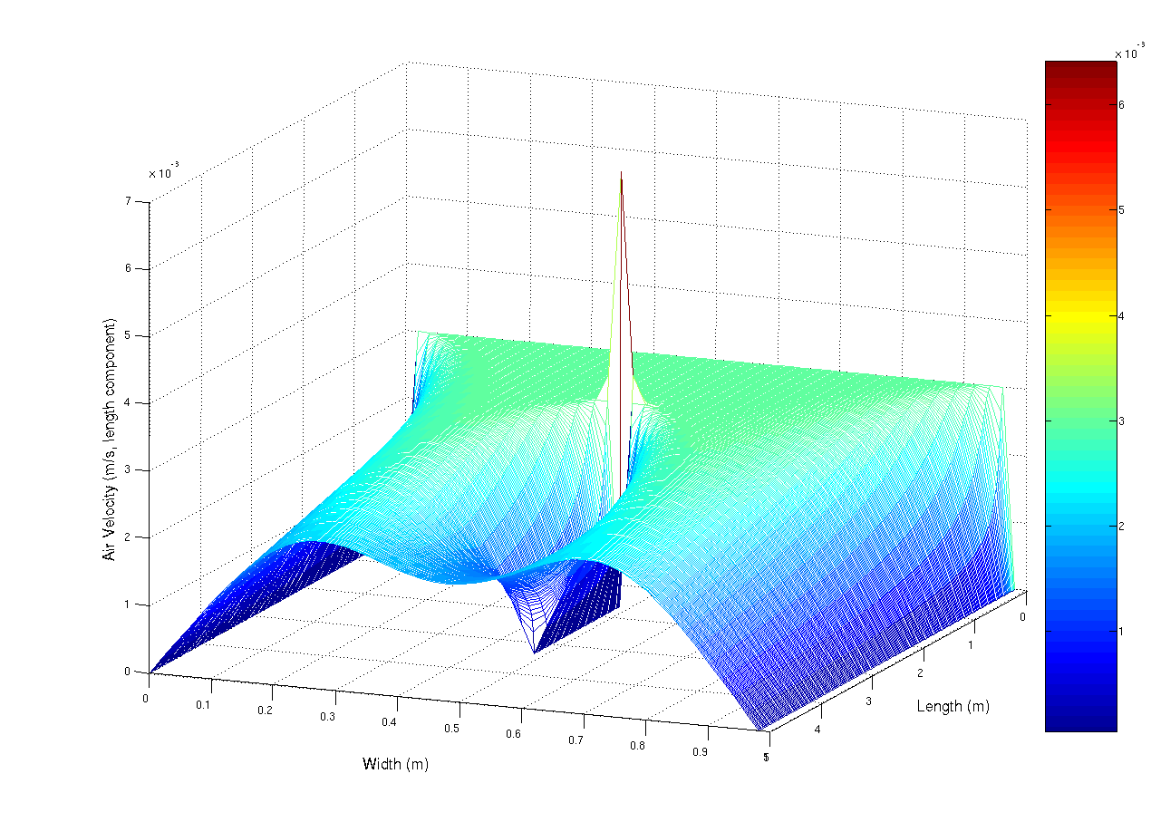
A simulation using the navier-stokes differential equations of the aiflow into a duct at 0.003 m/s (laminar flow). The duct has a small obstruction in the centre that is parallel with the duct walls. The observed spike is mainly due to numerical limitations. This script, which i originally wrote for scilab, but ported to matlab (porting is really really easy, mainly convert comments % -> // and change the fprintf and input statements) Matlab was used to generate the image.
%Matlab script to solve a laminar flow
%in a duct problem

%Constants
inVel = 0.003; % Inlet Velocity (m/s)
fluidVisc = 1e-5; % Fluid's Viscoisity (Pa.s)
fluidDen = 1.3; %Fluid's Density (kg/m^3)

MAX_RESID = 1e-5; %uhh. residual units, yeah...
deltaTime = 1.5; %seconds?
%Kinematic Viscosity
fluidKinVisc = fluidVisc/fluidDen;

%Problem dimensions
ductLen=5; %m
ductWidth=1; %m

%grid resolution
gridPerLen = 50; % m^(-1)
gridDelta = 1/gridPerLen;
XVec = 0:gridDelta:ductLen-gridDelta;
YVec = 0:gridDelta:ductWidth-gridDelta;

%Solution grid counts
gridXSize = ductLen*gridPerLen;
gridYSize = ductWidth*gridPerLen;

%Lay grid out with Y increasing down rows
%x decreasing down cols
%so subscripting becomes (y,x) (sorry)
velX= zeros(gridYSize,gridXSize);
velY= zeros(gridYSize,gridXSize);
newVelX= zeros(gridYSize,gridXSize);
newVelY= zeros(gridYSize,gridXSize);

%Set initial condition

for i =2:gridXSize-1
for j =2:gridYSize-1
velY(j,i)=0;
velX(j,i)=inVel;
end
end

%Set boundary condition on inlet
for i=2:gridYSize-1
velX(i,1)=inVel;
end

disp(velY(2:gridYSize-1,1));

%Arbitrarily set residual to prevent
%early loop termination
resid=1+MAX_RESID;

simTime=0;

while(deltaTime)
 count=0;
while(resid > MAX_RESID && count < 1e2)
 count = count +1;
for i=2:gridXSize-1
for j=2:gridYSize-1
newVelX(j,i) = velX(j,i) + deltaTime*( fluidKinVisc / (gridDelta.^2) * ...
(velX(j,i+1) + velX(j+1,i) - 4*velX(j,i) + velX(j-1,i) + ...
velX(j,i-1)) - 1/(2*gridDelta) *( velX(j,i) *(velX(j,i+1) - ...
velX(j,i-1)) + velY(j,i)*( velX(j+1,i) - velX(j,i+1))));

newVelY(j,i) = velY(j,i) + deltaTime*( fluidKinVisc / (gridDelta.^2) * ...
(velY(j,i+1) + velY(j+1,i) - 4*velY(j,i) + velY(j-1,i) + ...
velY(j,i-1)) - 1/(2*gridDelta) *( velY(j,i) *(velY(j,i+1) - ...
velY(j,i-1)) + velY(j,i)*( velY(j+1,i) - velY(j,i+1))));
end
end

%Copy the data into the front
for i=2:gridXSize - 1
for j = 2:gridYSize-1
velX(j,i) = newVelX(j,i);
velY(j,i) = newVelY(j,i);
end
end

%Set free boundary condition on inlet (dv_x/dx) = dv_y/dx = 0
for i=1:gridYSize
velX(i,gridXSize)=velX(i,gridXSize-1);
velY(i,gridXSize)=velY(i,gridXSize-1);

    end

    %y velocity generating vent
    for i=floor(2/6*gridXSize):floor(4/6*gridXSize)
        velX(floor(gridYSize/2),i) = 0;
        velY(floor(gridYSize/2),i-1) = 0;
    end

%calculate residual for
%conservation of mass
resid=0;
for i=2:gridXSize-1
for j=2:gridYSize-1
%mass continuity equation using central difference
%approx to differential
resid = resid + (velX(j,i+ 1)+velY(j+1,i) - ...
(velX(j,i-1) + velX(j-1,i)))^2;
end
end

resid = resid/(4*(gridDelta.^2))*1/(gridXSize*gridYSize);
fprintf('Time %5.3f \t log10Resid : %5.3f\n',simTime,log10(resid));


simTime = simTime + deltaTime;
end
mesh(XVec,YVec,velX)
deltaTime = input('\nnew delta time:');
end
%Plot the results
mesh(XVec,YVec,velX)
|
| Datum | 24. Februar 2007 (Original-Hochladedatum) |
| Quelle | Übertragen aus en.wikipedia nach Commons. |
| Urheber | User A1 in der Wikipedia auf Englisch |
Lizenz
| Dieses Werk wurde von seinem Urheber User A1 in der Wikipedia auf Englisch als gemeinfrei veröffentlicht. Dies gilt weltweit. In manchen Staaten könnte dies rechtlich nicht möglich sein. Sofern dies der Fall ist: User A1 gewährt jedem das bedingungslose Recht, dieses Werk für jedweden Zweck zu nutzen, es sei denn, Bedingungen sind gesetzlich erforderlich. |
Ursprüngliches Datei-Logbuch
- 2007-02-24 05:45 User A1 1270×907×8 (86796 bytes) A simulation using the navier-stokes differential equations of the aiflow into a duct at 0.003 m/s (laminar flow). The duct has a small obstruction in the centre that is paralell with the duct walls. The observed spike is mainly due to numerical limitatio
Dateiversionen
Klicke auf einen Zeitpunkt, um diese Version zu laden.
| Version vom | Vorschaubild | Maße | Benutzer | Kommentar | |
|---|---|---|---|---|---|
| aktuell | 17:52, 1. Mai 2007 | | 1.270 × 907 (85 KB) | Smeira | {{Information |Description=A simulation using the navier-stokes differential equations of the aiflow into a duct at 0.003 m/s (laminar flow). The duct has a small obstruction in the centre that is paralell with the duct walls. The observed spike is mainly |
Dateiverwendung
Die folgende Seite verwendet diese Datei:
Globale Dateiverwendung
Die nachfolgenden anderen Wikis verwenden diese Datei:
- Verwendung auf anp.wikipedia.org
- Verwendung auf ar.wikipedia.org
- Verwendung auf ba.wikipedia.org
- Verwendung auf bg.wikipedia.org
- Verwendung auf bn.wikipedia.org
- Verwendung auf ca.wikipedia.org
- Verwendung auf ckb.wikipedia.org
- Verwendung auf cs.wikipedia.org
- Verwendung auf en.wikipedia.org
- Verwendung auf en.wikiquote.org
- Verwendung auf es.wikipedia.org
- Verwendung auf fa.wikipedia.org
- Verwendung auf he.wikipedia.org
- Verwendung auf hif.wikipedia.org
- Verwendung auf hi.wikipedia.org
- Verwendung auf hr.wikipedia.org
- Verwendung auf hy.wikipedia.org
- Verwendung auf id.wikipedia.org
- Verwendung auf jv.wikipedia.org
- Verwendung auf ko.wikipedia.org
- Verwendung auf ko.wikiversity.org
- Verwendung auf map-bms.wikipedia.org
- Verwendung auf ms.wikipedia.org
- Verwendung auf mwl.wikipedia.org
- Verwendung auf pt.wikipedia.org
- Isaac Newton
- Equação diferencial
- Equações de Navier-Stokes
- Equação diferencial linear
- Equação diferencial de Bernoulli
- Equação diferencial de d'Alembert
- Decaimento exponencial
- Equação de Laplace
- Equação diferencial parcial
- Equação de Poisson
- Equação do calor
- Lema de Grönwall
- Teorema de Picard-Lindelöf
- Método de Runge-Kutta
- Equação de Mason-Weaver
- Equação do pêndulo
- Equação de onda
Weitere globale Verwendungen dieser Datei anschauen.