Datei:Bloop locations.png
Zur Navigation springen
Zur Suche springen
Größe dieser Vorschau: 600 × 600 Pixel. Weitere Auflösungen: 240 × 240 Pixel | 480 × 480 Pixel | 768 × 768 Pixel | 1.024 × 1.024 Pixel | 2.048 × 2.048 Pixel | 3.000 × 3.000 Pixel
Originaldatei (3.000 × 3.000 Pixel, Dateigröße: 7,74 MB, MIME-Typ: image/png)
![]()
Diese Datei und die Informationen unter dem roten Trennstrich werden aus dem zentralen Medienarchiv Wikimedia Commons eingebunden.
![]()
Beschreibung
| Beschreibung |
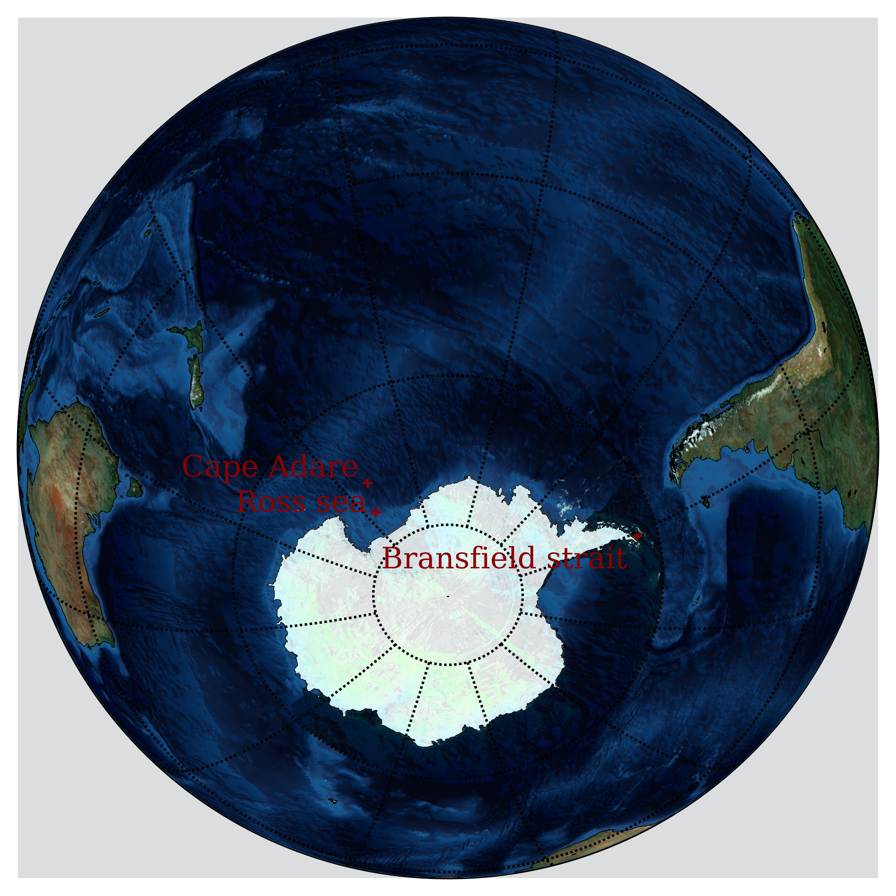
English: Possible locations of the Bloop, an ultra-low frequency and extremely powerful underwater sound detected by the U.S. National Oceanic and Atmospheric Administration (NOAA) in 1997. |
| Datum | |
| Quelle | Eigenes Werk |
| Urheber | Nojhan |
| PNG‑Erstellung | Diese PNG-Rastergrafik wurde mit Python erstellt. |
Source code
This image has been generated by the following source code in Python:
Python code
| source code |
|---|
print "import modules...",
import sys
sys.stdout.flush()
import pickle
from mpl_toolkits.basemap import Basemap, shiftgrid, cm
import matplotlib
import matplotlib.pyplot as plt
import numpy as np
from netCDF4 import Dataset
print "ok"

# Lovecraft: 47:9'S 126:43'W
# lovecraft_lat = -47.9
# lovecraft_lon = -126.43

# August Derleth: 49:51'S 128:34'W
# derleth_lat = -49.51
# derleth_lon = -128.34

# Nemo point: 48:52.6'S 123:23.6'W
# nemo_lat = -48.526
# nemo_lon = -123.236

# The Bloop:
bransfield_strait_lat=-63
bransfield_strait_lon=-59
ross_sea_lat = -75
ross_sea_lon = -175
cape_adare_lat = -71.17
cape_adare_lon = -170.14

mid_lat = np.mean((bransfield_strait_lat,ross_sea_lat,cape_adare_lat))
mid_lon = np.mean((bransfield_strait_lon,ross_sea_lon,cape_adare_lon))


# Not necessary, because the default projection is ortho,
# but can be useful if you want another one.
def equi(m, centerlon, centerlat, radius, *args, **kwargs):
    """
    Drawing circles of a given radius around any point on earth, given the current projection.
    http://www.geophysique.be/2011/02/20/matplotlib-basemap-tutorial-09-drawing-circles/
    """
    glon1 = centerlon
    glat1 = centerlat
    X = []
    Y = []
    for azimuth in range(0, 360):
        glon2, glat2, baz = shoot(glon1, glat1, azimuth, radius)
        X.append(glon2)
        Y.append(glat2)
    X.append(X[0])
    Y.append(Y[0])

    #m.plot(X,Y,**kwargs) #Should work, but doesn't...
    X,Y = m(X,Y)
    plt.plot(X,Y,**kwargs)


def shoot(lon, lat, azimuth, maxdist=None):
    """Shooter Function
    Plotting great circles with Basemap, but knowing only the longitude,
    latitude, the azimuth and a distance. Only the origin point is known.
    Original javascript on http://williams.best.vwh.net/gccalc.htm
    Translated to python by Thomas Lecocq :
    http://www.geophysique.be/2011/02/19/matplotlib-basemap-tutorial-08-shooting-great-circles/
    """
    glat1 = lat * np.pi / 180.
    glon1 = lon * np.pi / 180.
    s = maxdist / 1.852
    faz = azimuth * np.pi / 180.

    EPS= 0.00000000005
    if ((np.abs(np.cos(glat1))<EPS) and not (np.abs(np.sin(faz))<EPS)):
        alert("Only N-S courses are meaningful, starting at a pole!")

    a=6378.13/1.852
    f=1/298.257223563
    r = 1 - f
    tu = r * np.tan(glat1)
    sf = np.sin(faz)
    cf = np.cos(faz)
    if (cf==0):
        b=0.
    else:
        b=2. * np.arctan2 (tu, cf)

    cu = 1. / np.sqrt(1 + tu * tu)
    su = tu * cu
    sa = cu * sf
    c2a = 1 - sa * sa
    x = 1. + np.sqrt(1. + c2a * (1. / (r * r) - 1.))
    x = (x - 2.) / x
    c = 1. - x
    c = (x * x / 4. + 1.) / c
    d = (0.375 * x * x - 1.) * x
    tu = s / (r * a * c)
    y = tu
    c = y + 1
    while (np.abs (y - c) > EPS):

        sy = np.sin(y)
        cy = np.cos(y)
        cz = np.cos(b + y)
        e = 2. * cz * cz - 1.
        c = y
        x = e * cy
        y = e + e - 1.
        y = (((sy * sy * 4. - 3.) * y * cz * d / 6. + x) *
              d / 4. - cz) * sy * d + tu

    b = cu * cy * cf - su * sy
    c = r * np.sqrt(sa * sa + b * b)
    d = su * cy + cu * sy * cf
    glat2 = (np.arctan2(d, c) + np.pi) % (2*np.pi) - np.pi
    c = cu * cy - su * sy * cf
    x = np.arctan2(sy * sf, c)
    c = ((-3. * c2a + 4.) * f + 4.) * c2a * f / 16.
    d = ((e * cy * c + cz) * sy * c + y) * sa
    glon2 = ((glon1 + x - (1. - c) * d * f + np.pi) % (2*np.pi)) - np.pi

    baz = (np.arctan2(sa, b) + np.pi) % (2 * np.pi)

    glon2 *= 180./np.pi
    glat2 *= 180./np.pi
    baz *= 180./np.pi

    return (glon2, glat2, baz)


print "read in etopo5 topography/bathymetry"
url = 'http://ferret.pmel.noaa.gov/thredds/dodsC/data/PMEL/etopo5.nc'
etopodata = Dataset(url)

print "get data"

def topopickle(etopodata,name):
    import sys
    print "\t"+name+"...",
    sys.stdout.flush()
    filename = "rlyeh_"+name+".pickle"
    try:
        with open(filename,"r") as fd:
            print "load...",
            var = pickle.load(fd)
    except IOError:
        print "copy...",
        var = etopodata.variables[name][:]
        with open(filename,"w") as fd:
            print "dump...",
            pickle.dump(var,fd)
    print "ok"
    return var

topoin = topopickle(etopodata,"ROSE")
lons   = topopickle(etopodata,"ETOPO05_X")
lats   = topopickle(etopodata,"ETOPO05_Y")
print "shift data so lons go from -180 to 180 instead of 20 to 380...",
sys.stdout.flush()
topoin,lons = shiftgrid(180.,topoin,lons,start=False)
print "ok"


# create the figure and axes instances.
fig = plt.figure()
ax = fig.add_axes([0.1,0.1,0.8,0.8])

print "setup basemap"
# set up orthographic m projection with
# perspective of satellite looking down at 50N, 100W.
# use low resolution coastlines.
m = Basemap(projection='ortho',lat_0=mid_lat,lon_0=mid_lon,resolution='l')
m.bluemarble()

# Generic Mapping Tools colormaps:
# GMT_drywet, GMT_gebco, GMT_globe, GMT_haxby GMT_no_green, GMT_ocean, GMT_polar,
# GMT_red2green, GMT_relief, GMT_split, GMT_wysiwyg

print "transform to nx x ny regularly spaced native projection grid"
# step=5000.
step=10000.
nx = int((m.xmax-m.xmin)/step)+1; ny = int((m.ymax-m.ymin)/step)+1
topodat = m.transform_scalar(topoin,lons,lats,nx,ny)

print "plot topography/bathymetry as shadows"
from matplotlib.colors import LightSource
ls = LightSource(azdeg = 45, altdeg = 220, hsv_min_val=0.0, hsv_max_val=1.0,
        hsv_min_sat=0.0, hsv_max_sat=1.0)
# convert data to rgb array including shading from light source.
# (must specify color m)
rgb = ls.shade(topodat, cm.GMT_ocean)
im = m.imshow(rgb, alpha=0.15)

print "draw coastlines, country boundaries, fill continents"
m.drawcoastlines(linewidth=0.25)
# draw the edge of the map projection region
m.drawmapboundary(fill_color='white')
# draw lat/lon grid lines every 30 degrees.
m.drawmeridians(np.arange(  0,360,30), color="black" )
m.drawparallels(np.arange(-90,90 ,30), color="black" )

print "draw points"
psize=5
font = {'family' : 'serif',
        'weight' : 'normal',
        'size'   : 12}
matplotlib.rc('font', **font)

# x,y = m( lovecraft_lon, lovecraft_lat )
# m.scatter(x,y,psize,marker='o', color='white')
# plt.text(x+50000,y+50000+50000, "Lovecraft", color='white')
#
# x,y = m( derleth_lon, derleth_lat )
# m.scatter(x,y,psize,marker='o',color='white')
# plt.text(x+50000-120000,y+50000, "Derleth", color='white', horizontalalignment="right")

# x,y = m( nemo_lon, nemo_lat )
# m.scatter(x,y,psize*3,marker='+',color='#555555')
# plt.text(x+50000+50000,y+50000-80000, "Nemo", color="#555555", verticalalignment="top")
#
# equi(m, nemo_lon, nemo_lat, radius=2688, color="#555555" )

pcolor="darkred"
offset=150000

x,y = m( bransfield_strait_lon, bransfield_strait_lat )
m.scatter(x,y,psize*3,marker='+',color=pcolor)
plt.text(x-offset,y-offset, "Bransfield strait", color=pcolor,
        horizontalalignment="right", verticalalignment="top")

x,y = m( ross_sea_lon, ross_sea_lat )
m.scatter(x,y,psize*3,marker='+',color=pcolor)
plt.text(x-offset,y, "Ross sea", color=pcolor,
        horizontalalignment="right", verticalalignment="bottom")

x,y = m( cape_adare_lon, cape_adare_lat )
m.scatter(x,y,psize*3,marker='+',color=pcolor)
plt.text(x-offset,y, "Cape Adare", color=pcolor,
        horizontalalignment="right", verticalalignment="bottom")

plt.savefig("Bloop_locations.png", dpi=600, bbox_inches='tight')
# plt.show()
|
Lizenz
Ich, der Urheber dieses Werkes, veröffentliche es unter der folgenden Lizenz:
Diese Datei ist unter der Creative-Commons-Lizenz „Namensnennung – Weitergabe unter gleichen Bedingungen 3.0 nicht portiert“ lizenziert.
- Dieses Werk darf von dir
- verbreitet werden – vervielfältigt, verbreitet und öffentlich zugänglich gemacht werden
- neu zusammengestellt werden – abgewandelt und bearbeitet werden
- Zu den folgenden Bedingungen:
- Namensnennung – Du musst angemessene Urheber- und Rechteangaben machen, einen Link zur Lizenz beifügen und angeben, ob Änderungen vorgenommen wurden. Diese Angaben dürfen in jeder angemessenen Art und Weise gemacht werden, allerdings nicht so, dass der Eindruck entsteht, der Lizenzgeber unterstütze gerade dich oder deine Nutzung besonders.
- Weitergabe unter gleichen Bedingungen – Wenn du das Material wiedermischst, transformierst oder darauf aufbaust, musst du deine Beiträge unter der gleichen oder einer kompatiblen Lizenz wie das Original verbreiten.
Dateiversionen
Klicke auf einen Zeitpunkt, um diese Version zu laden.
| Version vom | Vorschaubild | Maße | Benutzer | Kommentar | |
|---|---|---|---|---|---|
| aktuell | 23:46, 12. Feb. 2013 | | 3.000 × 3.000 (7,74 MB) | Nojhan | User created page with UploadWizard |
Dateiverwendung
Die folgende Seite verwendet diese Datei:
Globale Dateiverwendung
Die nachfolgenden anderen Wikis verwenden diese Datei:
- Verwendung auf eo.wikipedia.org
- Verwendung auf es.wikipedia.org
- Verwendung auf fr.wikipedia.org
- Verwendung auf id.wikipedia.org
- Verwendung auf it.wikipedia.org